There are several choices of weight functions, ![]() . The most basic,
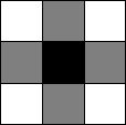
that we have opted to use, is that of the neighbourhood of 4 most adjacent positions,
as shown by the dark grey in Figure 1, with each position
being weighted
. The most basic,
that we have opted to use, is that of the neighbourhood of 4 most adjacent positions,
as shown by the dark grey in Figure 1, with each position
being weighted ![]() relative to the other positions.
relative to the other positions.
Another possibility is that of taking the most adjacent positions and the diagonally
adjacent positions, as shown by the dark and light grey in Figure 1.
Here, each of the most adjacent positions would have a relative weight of ![]() and each of the diagonally opposite positions would have a relative weight of
and each of the diagonally opposite positions would have a relative weight of
![]() , this way the sum of the weights is still unity and no scaling
of the central pixel value occurs.
, this way the sum of the weights is still unity and no scaling
of the central pixel value occurs.

|
Note that the 26 element, three dimensional neighbourhood is not necessarily
a better neighbourhood to take than the above 8 element two dimensional neighbourhood.
While all 26 elements are still local to the central position, the microscopes
that create these images usually do so in a layered fashion, that is, they scan
a layer of fixed ![]() at a time. Thus weighting functions are better taken
where all the elements considered are within a single, two dimensional layer
of fixed
at a time. Thus weighting functions are better taken
where all the elements considered are within a single, two dimensional layer
of fixed ![]() .
.